Chemical Potential

The Chemical Potential: Simple Thermodynamics of Chemical Processes

The chemical potential $\mu$, which is simply the free energy per molecule, is probably the most useful thermodynamic quantity for describing and thinking about chemical systems. Because $\mu$ represents an energy for one molecule, it is easy to think about concretely. In fact, for a system consisting of molecule types A, B, C, etc., each occurring with $N_A$, $N_B$, ... copies, we can write the total free energy at constant pressure exactly as

(1)

To focus on the chemical potential itself, we can say that $\mu_X$ is the energy required to add a molecule of type X to a system at temperature $T$ and pressure $P$, which consists of $N_A$ molecules of type A, $N_B$ molecules of type B, and so on. Importantly, the chemical potential is not a physical constant: implicit in $\mu$ are its many dependences

(2)

which often may not be written out. The key point is that, in general, the chemical potential depends on everything about the system. To give a simple example of such dependence, molecule type A could represent protons in solution (implying a certain pH), which would affect the energy required to add an acidic molecule of type B. As another example, in a solution of charged molecules of type A, the chemical potential $\mu_A$ will depend on how many A molecules are already present (i.e., the concentration [A]) because charged molecules repel one another. Note that the apparently simple form of Eq. (1) does not imply the molecule types are independent of one another because the $\mu$ values change as the $N$ values do.

To understand chemical equilibrium, a fundamental reference point in biochemistry, it turns out to be important to write the chemical potential as a derivative of the free energy. From the definition above, we want to know the incremental change in free energy $\Delta G$ based on adding a single molecule of type X - i.e., for $\Delta N_X = 1$. Using basic calculus ideas, we can write

(3)

Chemical reactions: Equilibrium and beyond

The chemical potential, by design, is the perfect tool for analyzing chemical behavior. Let us first consider the very simplest chemical reaction:

(4)

When getting started with a new system, it's always a good plan to examine the equilibrium point. Because the free energy will be minimized with respect to adjustable paramters ($N_A$ and $N_B$ in this case) at equilibrium, we should differentiate $G$ with respect to either $N_A$ or $N_B$. In fact, there is really only one adjustable parameter in this system since $N_B = N - N_A$ and $N$ is assumed constant. Using the basic rules of calculus and the definition of $\mu$ (3), we find

(6)

because $ d N_B / d N_A = -1$ at fixed total $N$. The equilibrium point itself is obtained by setting the $G$ derivative to zero (to minimize $G$), yielding the key chemical result that chemical potentials will match in equilibrium:

(8)

This equality of chemical potentials does not imply that $N_A = N_B$ at equilibrium: in general, the equilibrium point will imply quite different reactant and product numbers (and hence concentrations). After all, most reactions substantially favor either products or reactants under a given set of conditions.

Connection to reaction rates, free energy, and standard free energy

The chemical potential must be intimately related to reaction rates and standard free energies, which also can be said to "control" chemical reactions. We will begin to clarify those connections now. Briefly, the standard free energy indicates where the equilibrium point of a reaction will be, as does the ratio of reaction rate constants. The difference in chemical potentials, like the free energy difference (compared to the standard free energy) tells us about the displacement from equilibrium.

We'll start with the standard free energy change of reaction $\dgstd$, where the "$\circ$" indicates standard temperature and pressure and the prime (') denotes pH = 7. From any chemistry or biochemistry book, the definition (for our simple $A \rightleftharpoons B$ reaction) is

(9)

where it's essential to realize that this applies to the equilibrium concentrations at standard conditions. The second line defines the equilibrium constant $\kkeq = \conceq{B} / \conceq{A}$.

Eq. (9) tells us the precise relation between the equilibrium concentrations and the standard free energy. When the product (B) is "favored" (i.e., when $\conceq{B} > \conceq{A}$), then $\dgstd$ is negative, but when reactant A is favored then $\dgstd$ is positive. Turning that around, $\dgstd$ merely tells us the relative A and B concentrations that will occur at equilibrium. As we will see below, $\dgstd$ absolutely does not indicate whether a given reaction will tend to proceed in the forward direction, because that depends on the immediate (starting) species concentrations - which typically are not in equilibrium. Again, $\dgstd$ only indicates what the ratio of concentrations will be at equilibrium.

From the detailed-balance condition of equilibrium, we know that the ratio of rate constants also yield the equilibrium ratio of concentrations.

(10)

where $k_+$ is the rate constant for the A to B direction and $k_-$ is for the reverse reaction. This enables to write the standard free energy change in term of rates constants:

(11)

Using the explicit dependence of chemical potential on concentration, namely $\mu_X = \mu^{\circ}_X + RT \ln \conc{X}$ derived below in Eq. (27) assuming independent molecules, we can also re-write the equality of chemical potentials (8) in equilibrium as

(12)

Rearranging and comparing to the defintion of $\dgstd$ from Eq. (9), we have

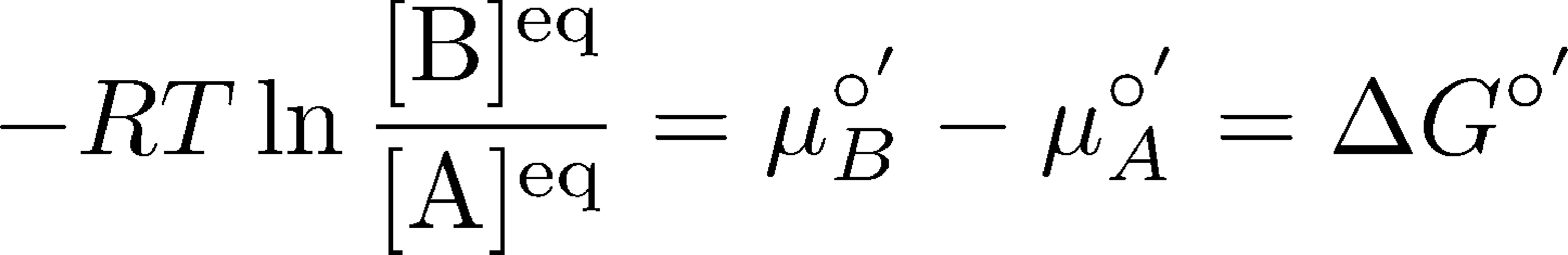(13)

where again the prime (') indicates we are considering pH = 7. It is very useful to also be familiar with exponentiated form of this same relation:

(14)

which makes it simpler to grasp that higher standard free energy of B (relative to A) decreases the relative equilibrium concentration of B, as shown in the figure by the green equilibrium horizontal tie lines.

We have now seen the full set of equilibrium connections among the chemical potential, standard free energy difference, and reaction rates. Most importantly, the standard free energy difference (and standard chemical potentials) merely set the equilibrium point. A lower standard chemical potential means a larger equilibrium concentration, as we see from Eq. (13).

Below, we will generalize these results for more complicated reactions.

What $\mu$ tells us about out-of-equilibrium systems

Biological systems are rarely in equilibrium, so it is essential to understand non-equilibrium behavior. The result (8) that chemical potentials match in equilibrium is equally valuable for what it tells us about systems which are out of equilibrium, namely, that the chemical potentials are not equal. Such non-equilibrium systems will always tend to be driven toward equilibrium.

Consider a case where $\mu_A > \mu_B$ (so $\Delta \mu = \mu_B - \mu_A < 0$), and assume the chemical potential depends on concentration according to Eq. (27), derived below. Then we have

(15)

which can be re-written as

(16)

That is, in this particular non-equilibrium example, the concentration of A is (relatively) higher than its equilibrium value: compare to Eq. (14). As shown in the figure below, for a non-equilibrium reaction with $\Delta \mu < 0$, the concentrations of A and B differ from the equilibrium values which would be described by a horizontal tie line (equal $\mu$ values).

steady state.

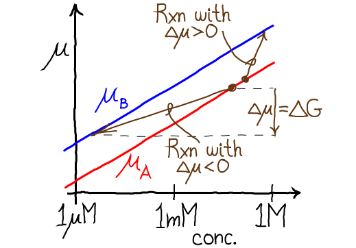
Importantly, the chemical potential difference $\Delta \mu = \mu_B - \mu_A$ tells us the actual free energy required (or released, if negative) when a reaction occurs at a specific set of conditions - which is absolutely critical for understanding cellular reactions such as the hydrolysis of ATP under cellular conditions. (Remember that the standard free energy change $\dgstd$ only tells us the equilibrium point and not the free energy change for a realistic reaction.) When $\Delta \mu = 0$, we have equilibrium, and no free energy is required to push the reaction. The figure shows two examples of non-equilibrium reactions: the vertical components of the brown arrows represent the $\Delta \mu$ values in each case.

Using Eq. (27), we can write the independent-molecule approximation for the change in chemical potential which is precisely equal to $\Delta G$ for the reaction, which can be seen from Eq. (1) for a single reaction which corresponds to $\Delta N_B = - \Delta N_A = 1$ since one A molecule is converted to B.

(17)

You can probably guess that $\Delta \mu$ for ATP hydrolysis is large and negative under typical cellular conditions though it can take on any value - even positive - under different conditions. Of course, the cell has tricks for making unfavorable reactions ($\Delta \mu > 0$) occur - by coupling them to other reactions that are more favorable still, so that the overall $\Delta \mu$ is negative.

More complex reactions

The book by Hill or any chemical thermodynamics text will explain the full generalization of the preceding results. Here we consider a somewhat more general reaction that will be useful for nucleotides, namely,

(18)

with forward and reverse rate constants $k_+$ and $k_-$. A key example is ATP + H$_2$O $\rightleftharpoons$ ADP + Pi.

By applying mass-action kinetic rules to the reaction (18), we obtain the equilibrium balance condition $\conceq{A} \conceq{B} k_+ = \conceq{C} \conceq{D} k_-$, that in turn can be rewritten as

(19)

The free energy per reaction under non-equilibrium conditions (typical of the cell) can be derived following Eqs. (1) and (17). For the reaction (18), we have

(20)

which is the free energy change per reaction in the forward direction. Thus, for example, if the concentrations of C and D exceed their equilibrium values, then the free energy change is positive - take the log of Eq. (19) to see this. A positive free energy change for a reaction implies that free energy is required for the reaction to occur. In other words, on average, the reaction will occur spontaneously only in reverse, which makes sense since the level of "products" (C and D) is elevated.

ATP free energy under cellular conditions

ATP is famously the fuel of the cell, but to understand this quantitatively - or even in a qualitatively accurate way - we need to use the free energy and chemical potential concepts developed here. The ATP hydrolysis reaction is

(21)

with $\dgstd = -7.3$ kcal/mol (which refers to the forward/hydrolysis direction) according to Berg's textbook. That is, under standard conditions ADP is favored over ATP - i.e., in equilibrium the concentration of ADP will greatly exceed that of ATP - given typical water and phosphate concentrations. In the cell, however, there is often more ATP than ADP, leading to an even larger (more negative) $\Delta G \simeq - 12$ kcal/mol via Eq. (20).

To understand this mathematically, we can re-cast Eq. (20) for ATP hydrolysis using Eq. (19) as

(22)

where we have used the fact that the concentration of water will change only negligibly due the reaction. If $\Delta G \simeq - 12$ kcal/mol, that means that the cellular concentrations (numerator) differ from the equilibrium concentrations (denominator) by more than seven orders of magnitude! It is in this sense only that ATP is a highly activated molecule: the concentrations are kept far from equilibrium. Even though $\dgstd$ is large and negative, if the cellular concentrations matched the equilibrium values there would be no usable $\Delta G$.

The figure shows the free energy considerations for ATP hydrolysis in a very schematic way - assuming the concentrations of water and phosphate are constant (though [Pi] certainly would change significantly). Qualitatively, the figure gives a correct sense of hydrolysis free energetics: the red ADP chemical potential is well below that for ATP (blue), and for cellular hydrolysis the actual free energy change per reaction is greater than the vertical distance ($\dgstd$ for standard conditions) because cellular [ATP] typically exceeds [ADP].

The immediate energy source for synthesis of ATP - addition of phosphate to ADP - is a proton electrochemical gradient in most cells. The phosphorylation is accomplished by the ATP synthase using a remarkable series of free energy transductions, from chemical to mechanical, and back to chemical energy.

Deriving the (approximate) anayltical form for the chemical potential

Building on our statistical mechanics discussion of the ideal gas, we can derive an equation for the chemical potential of a system of molecules, under the assumption they do not interact with one another. In this sense, the molecules are "ideal" in the same way as ideal gas particles. To fully appreciate the brief derivation below, readers should first review the partition function calculation in the ideal gas section.

Without writing down all the details, for $N$ non-interacting molecules of type X in a fixed volume V, the partition function becomes

(23)

where the dimensionless factor $q_X$ (which does not appear in the simple ideal gas partition function) represents integration of the Boltzmann factor over all degrees of freedom internal to the molecule - bond lengths, angles, and dihedrals. Thus, $q_X$ is an internal partition function which may include substantial intra-molecular interactions, but any inter-molecular interactions are neglected. Note that the factorized form (23) is expected for non-interacting/independent species because the energy in the Boltzmann factor does not connect different molecules; separating the center-of-mass behavior as the usual ideal gas factors is simply a mathematical trick: see, e.g., books by Hill and Zuckerman for further details.

We can derive the free energy itself, using the relation $F = -k_B T \ln Z$ along with Stirling's approximation, which leads to

(24)

Although we will not prove it here, the chemical potential can be derived either by differentiating the Gibbs free energy $G$ or the Helmholtz free energy $F$. The two will be equivalent when volume fluctuations are not important, which is what we expect for systems of biological interest, which tend to contain a large number of reactant and product molecules. (See the book by Zuckerman for more detailed discussion of volume fluctuations.) Assuming this equivalence, we have

(25)

It is convenient to separate this out into two terms using the rules of logarithms:

(26)

where we have explicitly shown the standard one molar ("1M") concentration which makes arguments of the logs dimensionless and also makes the first term the standard chemical potential $\mu^{\circ}_X = k_B T \ln \left( \mbox{1M} \lambda_X^3 / q_X \right)$. The full chemical potential is then, in molar energy units

(27)

References

- T.L. Hill, An Introduction to Statistical Thermodynamics, Dover, 1986.
- J. M. Berg et al., "Biochemistry", W. H. Freeman. The 2002 edition is online for free.
- D.M. Zuckerman, Statistical Physics of Biomolecules: An Introduction (CRC Press, 2010).
Exercises
- Explain the quantitative relationship between $k_B T$ which uses the Boltzmann constant and $RT$ which uses the gas constant. To do this, convert $k_B T$ in MKS units for $T$ = 300K to units of kcal/mole.
- For the reaction A + B $\rightleftharpoons$ C, starting from the explicit form of the Gibbs free energy (1), derive the equilibrium relation $\mu_A + \mu_B = \mu_C$. Use the fact that $N_C$ must increase when $N_A$ and $N_B$ decrease.