Active ("Kinetic") Proofreading
Primary tabs
One of the most remarkable tasks accomplished by the cell is the exchange of energy for information, as originally hypothesized in separate works by Hopfield and Ninio. That is, the cell performs processes like transcription (of DNA to mRNA) and translation (of mRNA to protein) with greater fidelity than would be possible if it only relied on binding affinity to attach the correct base or amino acid. The cell achieves this using "proofreading" processes that are driven by the expenditure of free energy. These processes conventionally are described as kinetic proofreading though driven or active proofreading would be terminology more consistent with discussions presented in these pages - e.g., active vs. passive transport.
We will study proofreading which occurs in the translation process - in the synthesis of protein based on an mRNA sequence. The source of free energy turns out to be the activated carrier GTP rather than ATP.
The figure schematically demonstrates the translation process occurring in a cell. The ribosome is the molecular machine responsible for translation. Starting in the upper left (state 1), the ribosome links a tRNA molecule bound with an amino acid (AA) to a complex including the preceding two tRNA molecules and the growing polypeptide chain. The incoming tRNA/AA molecules are complexed to an EF protein which is also bound to GTP. GTP hydrolysis drives the cycle in a counter-clockwise direction, adding a step (state 2) to the process which seems to be extraneous. In fact, the extra step is what makes proofreading possible by permitting a second opportunity for unbinding of tRNA/AA from the ribosome - which ultimately aids discrimination between correct and incorrect amino acids. From state 3, the polypeptide chain is extended by the formation of a covalent bond to the new AA; EF/GDP unbinds and the system yields state 4 which cannot receive a new tRNA/AA because the binding site is occupied. In a driven multi-step process not shown (grey arrow) the ribosome also translates the peptide chain and three tRNA molecules to the right, ejecting the rightmost tRNA which was added earliest.
Qualitative Picture of Proofreading: Penne vs. Bowties
How does proofreading work? Let’s imagine we have two types of cooked pasta, (tubular) penne and (relatively flat) bowties, which have different adhesive properties because of their shapes. Assume the two pastas are mixed together but we want to extract a batch that’s purely bowties. Because of their flatter shape, bowties are presumed to stick better to a flat surface.
In our thought experiment, we’ll place the pasta mixture in a cardboard box and shake it hard for a while. When we open the box, we’ll find that more bowties than penne are stuck to the box walls, because bowties just adhere better. The ratio of bowties to penne on the box wall is like the ratio of equilibrium populations – under the ‘thermal’ condition of box shaking.
Now for the proofreading. Imagine we cut out one wall from the box (with all the pasta intact) and place it in front of a powerful fan. The air blowing from the fan will apply an equal force to each piece of pasta. However, the penne has adhered more weakly and is more likely to fall off. Hence after the fan does its work, the ratio of bowties to penne on the cardboard wall will increase over its ‘equilibrium’ value … and we’ve accomplished proofreading! This is shown schematically in the image below, where red X’s mark the pasta blown off by the fan.

In a more abstract sense, when we have two species with different adhesion/binding strengths and we apply the same force/energy to unbinding both, we will enrich the stronger-binding species. We necessarily will reduce the bound amount of the stronger binder, but we will gain discrimination. The cell, evidently, is willing to pay the price of less efficient binding of the correct tRNA in order to have fewer errors.
A model for driven proofreading in translation
This subtle process is best studied with a specific model. Following Hopfield, we can construct a tractable model for driven/kinetic proofreading by slightly simplifying the process sketched above.

In this kinetic scheme, we have omitted the EF protein but retained GTP, which is critical as the activated carrier providing the driving force for proofreading. We have also further simplified the final step of covalent addition of the amino acid. The symbol "C" should be thought of as the correct amino acid, in contrast to the wrong amino acid "D" shown in the full model below.

Only by including the dual cycles with both C and D can we assess the discriminatory power of the model. That is, we will need to know the relative likelihoods for C and D to be incorporated into the polypeptide chain. Proofreading is discrimination, after all.
Model specifics
The model is specified according to the rates in the diagram above, where the notation follows Hopfield's paper. It is a standard mass action model: letters besides $k$ are used for the rate constants of different processes to avoid excessive sub- and super-scripts. The model has the following features and assumptions, again following Hopfield:
- The amino acid complexes for C and D are assumed to be equally available in solution, so $\conc{\cgtp} = \conc{\dgtp}$.
- The rates $m$, $m'$ and $w$ are identical for both the C and D processes.
- On-rates are also assumed to be the same for both processes, so that $k'_C = k'_D$ and $l'_C = l'_D$.
- Discrimination is assumed to occur via unbinding processes, with the more favorable C being slower to unbind compared to D. Specifically, off-rates are chosen to differ by a factor of $f_0 < 1$ so that $l_C = f_0 \, l_D$ and $k_C = f_0 \, k_D$.
- $\cgtp$ binding is assumed to be more favorable than $\cgdp$ binding, which can be realized via $l'_C < k'_C$, and similarly for D.
- The transition from RX to R$^*$X (with X = C or D) is assumed to be much slower than the RX unbinding processes: $m' \ll k_C, k_D$
- The rate $w$ for incorporating an amino acid onto the polypeptide chain (which involves multiple steps) is assumed to be much slower than all other rates.
You should recognize that, as with any cycle, there is a constraint which ensures thermodynamic consistency, so that only five of six rates are independent. This will be discussed further below.
An auxiliary cycle for activating the tRNA complexes
Although not essential for understanding the basics of driven proofreading, there is an additional cycle that governs the activation of the tRNA complexes: the unbinding of GDP and the binding of GTP to C or D. This activation cycle is interesting because it brings in the "raw" free energy associated with GTP hydrolysis/activation.
The C/GTP cycle is driven by the cell's continual synthesis of GTP. GTP is an activated carrier and its cellular concentration far exceeds its equilibrium value relative to the hydrolysis products GDP and Pi. An analogous cycle, with identical rate constants, is assumed for D/GTP binding and hydrolysis.
"Back-of-the-envelope" analysis
With only a few algebraic steps, and without including the auxiliary C/GTP cycle, we can demonstrate the basics of driven proofreading. In fact, for a quick analysis, it is easiest to exclude GTP and include driving only implicitly as will be described. Thus we consider a somewhat simplified cycle.

The rates shown in orange will later be used to model driving.
Translation without driving, roughly
First, let's consider the cycle "as is" with all rates/processes included. Because the rate $w$ is so slow (see above) and there is no driving, the cycles can be considered to be in equilibrium. In other words, all the processes happen so fast compared to the $w$ process that their relative populations are essentially equal to the equilibrium values. In this model, the equal availability of the two amino acid complexes amounts to assuming $\conc{C} = \conc{D}$.
Our goal is to calculate the discrimination ratio of correct (C) incorporation by the $w$ process to incorrect (D) incorporation in a steady state:
 (1)
(1)In the scenario just described, it is straightforward to solve for $\conc{\rstarx}$ using detailed balance along the right leg of each cycle. For the C cycle, we have $\conc{R} \conc{C} \, l'_C = \conc{\rstarc} \, l_C$ and similiar for D. Substituting into (1) and using assumptions stated above, we find
 (2)
(2)In other words, in this undriven scenario, discrimination occurs according the ratio of unbinding rates, which in turn is just the ratio of equilibrium dissociation constants because the on-rates are the same: see the discussion of binding.
Driven translation, roughly
To obtain a quick estimate of the effects of GTP-driving on the translation process, we will assume simply that the reverse processes shown in orange above are eliminated. That is, we will simply set the rate constants $m, l'_C, l'_D = 0$. You should recognize that this leads to an unphysical model (because detailed balance cannot be satisfied), but our goal is to construct a crude model of the effect of driving - without including the complications of the driving components. Don't worry - we will show later that the full model yields the same basic behavior as the simple version.
Procedurally, we will pursue a steady state analysis. We cannot use a quasi-equilibriium analysis, as we did for the undriven case, because we have explicitly put a net flow into the cycles by setting rate constants to zero.
In steady state, the net flow into every state balances the net flow out. For the $\mathrm{\rstarc}$ state, we have
 (3)
(3)where we used our assumption of very small $w$. The steady-state condition for the $\mathrm{\rdotc}$ state is
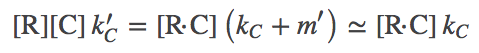 (4)
(4)where we again used one of our original assumptions that $m' \ll k_C$. Exactly analogous results are obtained for the D process.
We can combine the C and D steady state results to obtain the overall discrimination ratio. We use the preceding steady-state equations to solve for $\conc{\rstarc}$ in terms of $\conc{R}\conc{C}$, and similarly for D. From these steps we can obtain
 (5)
(5)where we used the original assumption $k'_C = k'_D$.
The driven discrimination ratio (5) is dramatically improved compared to the undriven case (2), when we recall that $f_0 < 1$. In a cellular context, $f_0$ can be as small as $1/100$ (see book by Alon) making driven proofreading 100 times better! Although we derived (5) using apparently unphysical assumptions, Hopfield has shown the same result is obtained from a full steady-state analysis. Our numerical data on the full model, below, are also consistent with the result.
Simulation of the full driven proofreading model
Simulation data is presented from the model specified below. Two cases were examined: afffinity ratios of $f_0 = 1/10, 1/100$. In both cases, simulations started from an initial condition where GTP (and hence $\cgtp$) was highly activated; simulations were run long enough so that $\cgtp$ became de-activated (via sufficient hydrolysis to GDP) and, accordingly, the proofreading became less driven.
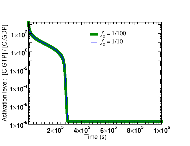
The first graph shows the time course of the de-activation of $\cgtp$, which is identical for both affinity ratios. The system is started in a highly activated non-equilibrium state and relaxes toward equilibrium.
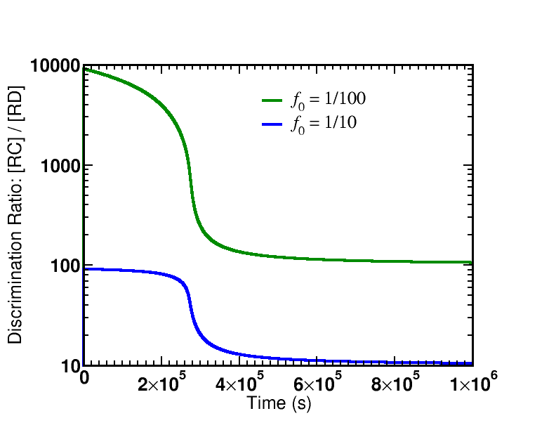
There are two key lessons from the figures plotting the discrimination ratio $\conc{RC} \left/ \conc{RD}\right.$: (i) The degree of discrimination decreases over time as GTP becomes de-activated, which is what we would expect. (ii) The discrimination ratio goes from a nearly maximal initial value $\sim 1/{f_0}^2$ as predicted by our simple analysis to the equilibrium value of $\sim 1/f_0$. Although it is not shown in the graphs, more than one GTP hydrolysis occurs per successful addition of amino acid in both cases.
The simulation data shown corresponds to an initial condition relaxing toward equilibrium, but it certainly is possible to run a non-equilibrium steady-state simulation in which GTP stays activated and the proofreading remains driven/active. This could be achieved by mimicking the cell's continual synthesis of GTP from GDP and Pi in a one-way reaction.
Rate constants for the model are specified below. Initial conditions were $\conc{GTP} = 10^{-3}$M, $\conc{GDP} = \conc{Pi} = 10^{-6}$M, $\conc{C} = \conc{D} = 10^{-4}$M, with 1,000 ribosomes (R). Simulations were performed using BioNetGen, a rule-based platform for kinetic modeling. The source code for the model (a .bngl file) can be downloaded by right-clicking here.
| Process | Symbol | Value |
|---|---|---|
| Reference on-rate | $\kon$ | $10^8$ / (M s) |
| Reference off-rate | $\koff$ | $100$ / s |
| Affinity ratio | $f_0$ | Adjustable parameter |
| $\cgtp$ binding | $k'_C$ | $\kon$ |
| $\cgtp$ unbinding | $k_C$ | $\koff$ |
| $\cgdp$ binding | $l'_C$ | $0.01 \, \kon$ |
| $\cgdp$ unbinding | $l_C$ | $\koff$ |
| GTP hydrolysis (Rib.) | $m'$ | $0.1 \, \koff$ |
| GTP synthesis (Rib.) | $m$ | cycle constraint (below) |
| Amino acid attachment | $w$ | $0.001 \, \koff$ |
| $\dgtp$ binding | $k'_D$ | $\kon$ |
| $\dgtp$ unbinding | $k_D$ | $\koff \left/ f_0\right.$ |
| $\dgdp$ binding | $l'_D$ | $0.01 \, \kon$ |
| $\dgdp$ unbinding | $l_D$ | $\koff \left/ f_0\right.$ |
| GTP binding | $g'_t$ | $\kon$ |
| GTP unbinding | $g_t$ | $\koff$ |
| GDP binding | $g'_d$ | $g'_t$ |
| GDP unbinding | $g_d$ | $10 \, \koff$ |
| GTP hydrolysis (aux.) | $k_h$ | $10^{-8} \, \koff$ |
| GTP synthesis (aux.) | $k_s$ | cycle constraint (below) |
Cycle constraints
Although we are studying processes far from equilibrium, we obtain important mathematical information about the rate constants by considering the equilibrium situation. This is because values of the rate constants are independent of conditions, equilibrium or otherwise (except in the case of an “external field,” possibly electrostatic, which is assumed not to play a role here). In other words, constants really are constant.
In our standard biochemical description, non-equilibrium processes arise because concentrations differ from their equilibrium values. For example, [GDP][Pi]/[GTP] will tend to be much smaller than its equilibrium value – i.e., GTP is activated. However, the rate constants are always the same, and this will hold so long as no fields are applied.
We will therefore analyze the cycles in our model in equilibrium. Accordingly, in the discussion immediately below, concentrations [X] really denote equilibrium concentrations [X]eq, although the superscript is omitted to keep the expressions cleaner. No specific concentration values will enter the final constraints – only equilibrium constants.
We first analyze the main cycle for ribosome (R) binding to $\cgtp$. As with any cycle, we apply detailed balance to each process and eliminate unwanted concentration terms to obtain
 (6)
(6)The right-hand side has the form of an equilibrium (dissociation) constant but it's not one we can look up in a biochemistry book. Instead we can express that constant in terms of the GTP constant by using the auxiliary cycle.
We therefore turn to the auxiliary cycle of C + GTP binding. From the detailed balance conditions, the constraint one finds is
 (7)
(7)where the right-hand side is the GTP hydrolysis equilibrium constant. However, we can also look directly at the detailed balance condition for GTP hydrolysis to find
 (8)
(8)
To get the relations into a useful form, we solve for the left-hand side of (8), namely $k_h / k_s$, from (7) and subtitute the result back into (8) to obtain
 (9)
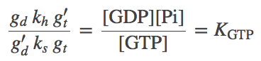
(9)This the result we want because it expresses the $\cgtp$ equilibrium constant in terms of a known equilibrium constant and rates from the model. Finally, we re-write (6) using (9) as
 (10)
(10)
Equations (7) and (10) are the constraints used to define missing model parameters, along with $K_{\mathrm{GTP}} = 5 \times 10^5$ M. The constraint for the R + $\dgtp$ cycle is analogous to (10).
Final thoughts: Does the cell really need driving for proofreading?

Take another look at the model for proofreading, and you may have the following epiphany: "Wait a second - we don't need driving for proofreading! We can just slow down all the processes for the wrong (D) substrate compared to C." This would be called "internal" proofreading, as opposed to external driven proofreading.
Indeed, it's true. Mathematically, we can easily raise the barriers (slow the rates) for the binding processes of R to the D complexes ... and that branch of the diagram would just get shut down. And there is evidence the cell does use some degree of internal proofreading. See, for example, the paper noted below by Banerjee et al. So why is there driving at all in cellular proofreading? Could a billion years of evolution have led to an unnecessary process?
One can speculate there are a couple of related reasons that driven proofreading is important in cells. First note that the task of discrimination is not merely to decide between two choices, but actually to choose only the correct substrate and nothing else - a challenging biochemical task. (When there are relatively few competing molecules, perhaps there is a larger role to be played by internal proofreading.) Suppose a molecular machine could arise with the ability to bind a target substrate with perfect physico-chemical complementarity but very weak affinity for even similar substrates. If such ideal "internal" discrimination were possible, the tightness of binding that would underlie it almost certainly would imply very slow kinetics. Thus, a high degree of internal discrimination suggests a very slow process that might not be useful to the cell.
Finally, note that the Hopfield scheme for kinetic proofreading presented here purposely excludes internal proofreading in order to illustrate the principles of driven proofreading. The goal has been to show how driving can (and apparently does) greatly expand the cell's ability to discriminate between target and off-target substrates.
Acknowledgement
A big thank you to Phil Nelson for carefully reading this page and requesting useful clarifications.
References
- B. Alberts et al., "Molecular Biology of the Cell," Garland Science (many editions available).
- K. Banerjee, A. B. Kolomeisky, and O.A. Igoshin, 2017. "Elucidating interplay of speed and accuracy in biological error correction." Proceedings of the National Academy of Sciences, 114:5183-5188 (2017).
- J. J. Hopfield, "Kinetic proofreading: A new mechanism for reducing errors in biosynthetic processes requiring high specificity," Proc. Nat. Acad. Sci. 71:4135-4139 (1974).
- J. Ninio, "Kinetic amplification of enzyme discrimination," Biochimie 57:587-595 (1975).
- U. Alon, An introduction to systems biology, CRC Press (2006).
Exercises
- Derive the constraint (6) among the rates for the R, RC, R$^*$C cycle.
- Derive the constraint (7) for the C/GTP "auxiliary" cycle. Show that the constraint from the previous cycle can be expressed in terms of rate constants from the C/GTP cycle.
- Derive the "back of the envelope" driven discrimination ratio (5).