Synthesis of ATP by ATP synthase
Primary tabs
Making the Miracle Molecule: ATP Synthesis by the ATP Synthase
ATP is the most important energized molecule in the cell. ATP is an activated carrier that stores free energy because it is maintained out of equilibrium with its hydrolysis products, ADP and Pi. There is a strong tendency for ATP to become hydrolyzed (split up) into ADP and Pi, and any process that couples to this reaction can be "powered" by ATP - even if that process would be unfavorable on its own. Examples include transport of other molecules across a membrane against the natural gradient and the action of motor proteins.

ATP is synthesized by a machine that may be even more remarkable, the ATP synthase (also called F-ATPase or FoF1-ATPase). As shown in the figure, the ATP synthase is an intricate rotary machine consisting of $\sim20$ proteins. The machine is driven by a difference in proton electrochemical potential across the bilayer (grey outline), which consists of both a pH difference (difference in proton concentrations) and an electrostatic potential - i.e., voltage - difference $\Delta \psi$. The proton-coupled free energy difference is sometimes called the "proton motive force" or pmf. The pmf drives proton transport (green arrows) from the positive P-side to the negative N-side of the membrane, which in turn causes rotation of the c-ring (brown) of the Fo subunit which is attached to the $\gamma$ stalk (brown). Rotation of the asymmetric $\gamma$ stalk within the three catalytic $\alpha \beta$ domains (light blue) of the F1 subunit suppplies energy sufficient for the synthesis of ATP - more precisely, for the phosophorylation of ADP.
In overview, an electrochemical gradient for protons is transduced into mechanical motion (rotation) which in turn creates sufficient conformational energy (elastic and perhaps electrostatic) to enable the highly unfavorable chemical reaction snythesizing ATP. This is fairly incredible.
Thermodynamic analysis of ATP synthesis
We can understand the driving forces through which the ATP synthase works without detailed knowledge or assumptions regarding structural details of the machine. For example, although mechanical/conformational free energy is transiently stored during the synthesis cycle, that is part of the inner workings of the machine that does not affect the overall thermodynamics. This is because all molecular machines are "passive devices" that reset to the exact same state after a cycle - in essence, machines simply are catalysts for complicated processes that may involve both chemical reactions and transport. The machines themselves do not supply energy but rather use free energy stored in other sources, such as activated carriers like ATP or concentration gradients.
The ATP synthase always generates three ATP molecules in a complete 360-degree rotational cycle because of the three catalyic $\alpha \beta$ domains, but the number of protons $n$ transported (which depends on the number of c-subunits - see figure above) varies from 8 to 15, depending on the organism and/or organelle. The overall "reaction" catalyzed by the ATP synthase (omitting water) is therefore

where "P" denotes the positive side of the membrane where the proton chemical potential is higher, and "N" is the "negative" side of lower chemical potential.
The overall free energy change per ATP synthesized is therefore the sum of the change in chemical potential $\mu$ for $n/3$ protons and the free energy cost for phopshorylating ADP:

We know that the overall $\dgtot$ must be negative, because the process does occur. The negative $\Delta \mu$ term will outweigh the positive $\Delta G$ for phosphorylating ADP.
Although the individual terms cannot really be known exactly, we can approximate them reasonably using our usual ideal gas (ideal solution) framework. We will build on the detailed discussion found in the chemical potential section, where we explored the free energy of ATP hydrolysis, $\Delta G(\mbox{ATP} \rightarrow \mbox{ADP})$, which is simply the negative of the $\Delta G$ value we want. We therefore have

where $\conc{X}$ denotes the cellular concentration of molecule X and $\conceq{X}$ is the equilibrium concentration. ATP is an "activated carrier" of free energy because its concentration is maintained far from equilibrium ... by the action of the ATP synthase. The state of activation for ATP is equivalent to the condition that $\Delta G(\mbox{ADP} \rightarrow \mbox{ATP}) > 0$.
When equilibrium and typical cellular values for the concentrations are substituted into (3), one finds that $\Delta G(\mbox{ADP} \rightarrow \mbox{ATP}) \simeq 12$ kcal/mol, which is about 20 times the thermal energy ($RT$ or $k_BT$) and quite a significant amount of energy!
For ATP synthesis to proceed, we know the total $\dgtot$ in (2) must be negative, so the change in proton chemical potential must be large and negative:

where $n = 8$ for the mammalian ATP synthase. As noted above, there are two driving forces acting on the protons: (i) the electrostatic potential difference across the membrane $\Delta \psi$, which simply creates an electric field that exerts a force on the proton as you learned in high school physics, and (ii) the pH difference $\Delta$pH across the membrane which creates a diffusive force that tends to equalize concentrations because pH is simply a measure of concentration. A more complete discussion of membrane electrostatics is available.
We can quantify the preceding description of proton driving forces, the pmf, again within ideal solution theory, via

where $F$ is Faraday's constant which simply converts the potential difference $\Delta \psi$ into energy units for a single proton charge. To interpret the overall effect of these terms, we must know the conventions adopted for the "$\Delta$" terms: for pH, it is P-side pH value minus the N-side pH making $\Delta$pH negative; for $\psi$ it is the same directionality, so the N-side voltage is subtracted from the P-side's, making $\Delta \psi$ positive. The net result that both terms of $\Delta \mu (\plus{H})$ are negative by convention. Physically, the absolute value of $\Delta \mu (\plus{H})$ is the free energy available per proton transported down the electro-chemical gradient. Note that sometimes the electro-chemical potential difference is assigned the symbol $\Delta \tilde{\mu}$ to remind us that there is an electric field present.
A simple kinetic model for ATP synthesis

We can get a more concrete understanding for how the synthase will behave by building a simple mass action model which incorporates some of the key features of its behavior. To allow us to build a model based on a relatively small number of equations, we will essentially model the synthesis of a single ATP - in effect, we will model 120 out of the full 360 degrees of the rotary cycle. And given that restriction, we will want the number of protons $n$ to be divisible by 3. We will choose $n = 9$ which is close to the $n=8$ value for mammalian ATP synthases.
The model will attempt to mimic the rotary mechanism in the following sequence of steps, as shown in the figure. Starting from state 1, ADP and Pi will bind the synthase, leading to state 3. A proton will then bind from the P side of the membrane, leading to state 4, followed by proton unbinding to the N side and state 5. (Rotation is implicitly included in the transitions 3$\rightarrow$4 and 4$\rightarrow$5, though for concreteness the figure shows it occuring with the 4$\rightarrow$5 transition.) Proton binding, unbinding and rotation repeat two more times, leading to state 9. The transition to state 10 is the catalytic step yielding ATP, and then ATP unbinding occurs leaving the machine back in state 1. All the steps will be reversible as is true for the cycle for any molecular machine.
The mass-action equations governing the model's kinetics are straightforward to write down. Using the notation that $[i]$ is the population of the machine in state $i$, the first equation is:

where $k_{12}$ and $k_{1,10}$ are on-rates, while $k_{21}$ and $k_{10,1}$ are off-rates. The other equations take similar forms. For example,

where $\conc{\plus{H}(\mbox{N})}$ is the proton concentration on the N side, $k_{98}$ is an on-rate, $k_{89}$ is an off-rate, while $k_{9,10}$ and $k_{10,9}$ are the catalytic rates for synthesis and hydrolysis, respectively.
To fully specify the model, we need all the rate constants. Some are available from the literature and others can be estimated, which is a fairly technical process that will not be discussed here. (The parameters used in the numerical data shown below are given in the model file also available below.) However, it is worth noting that not all the rate constants can take arbitrary parameters because of the usual constraint that occurs with any cycle.
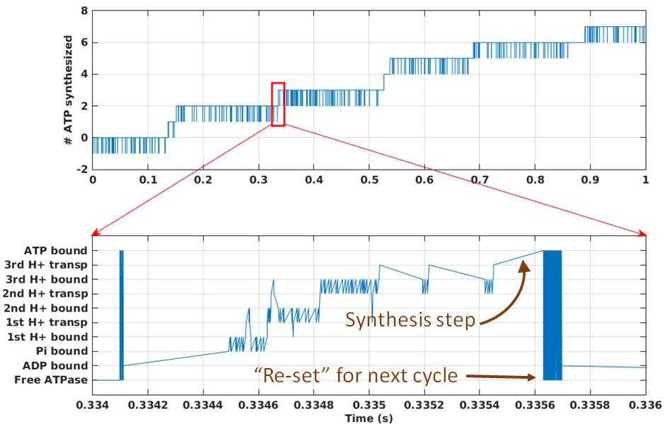
The figure shows stochastic simulation of our rotary model for a (molecular) time of 1 sec. Synthesis proceeds at a rate of about ~10 ATP/s, but note that there are frequent stochastic reversals. Such reversals, which occur at the level of overall ATP synthesis as driven by "microscopic" reversals among the 10 states we have set up, are expected to be an intrinsic part of the functioning of many molecular machines. On aggregate, however, with thousands of synthases per mitochondrion, there will be a very steady amount of synthesis at fixed driving conditions. The source code for the model (a .bngl file) can be downloaded here. The simulation was performed using BioNetGen, a rule-based platform for kinetic modeling.
Speed vs. efficiency and Synthesis vs. pumping
We can get a very useful overall understanding of the relation between the thermodynamics (driving free energy) and the kinetics of ATP synthesis by taking a closer look at Eq. (2). The equilibrium condition is when $\dgtot = 0$, so the driving free energy for the protons exactly balances the free energy necessary to phosphorylate ("synthesize") ATP:

In a plot of the chemical potential vs. the synthesis free energy, this corresponds to a straight line of slope $n/3$ as shown in the figure.
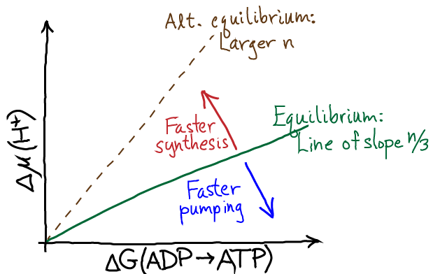
At equilibrium, there is zero net synthesis - which follows immediately from the balanced-flow definition of equilibrium. That is, while an occasional ADP might get phosphorylated by a synthase, that will be balanced out by an equal number of hydrolysis events. The further the system gets from equilibrium, the stronger the driving. With stronger driving we expect faster synthesis (in the region above the equilibrium line). There will be, however, a maximum speed at which the machine can operate, so ultimately the synthesis rate will level off even with very significant driving.
To visualize the relationship between thermodynamic driving and the ATP synthesis rate more quantiatively, it is useful to define the driving free energy as the negative of the total free energy chage, $\dgdrive = - \dgtot$. By convention, $\dgdrive$ is positive under synthesis conditions and negative for reverse operation of the synthase. In the figure below, the point marked with a red X represents the conditions used to generate the stochastic trajectories shown above.
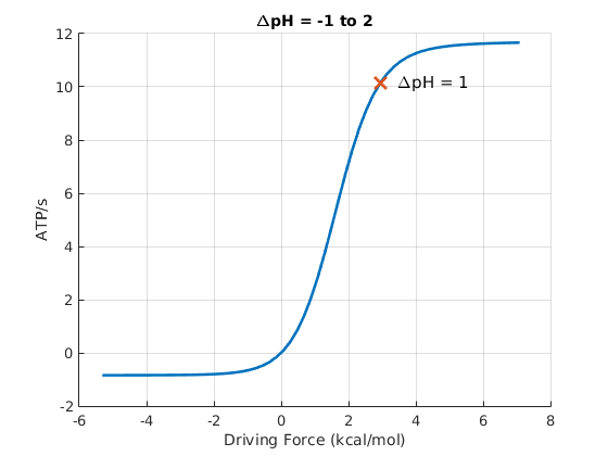
As with any molecular machine, the synthase can be driven in reverse, in which case it will act as a proton pump driven by ATP hydrolysis - as has been shown experimentally many times. The stronger the driving, the faster the pumping until the performance plateaus due to rate-limiting chemical and conformational steps. This behavior is seen in the figure for negative driving potential.
On the question of efficiency, Eq. (2) tells us that for any finite amount of driving, there must be some free energy "spilled" ($\dgtot$ is dissipated as heat) when synthesis proceeds at a finite rate. Hence, the efficiency - measured as the fraction of the proton free energy converted to ATP chemical free energy - is always less than 100%. The lower the driving, the higher the efficiency - at the price of reducing the speed of synthesis. The cell must optimize the tradeoff between speed and efficiency for its own purposes ... and note that some heat generation is not entirely wasteful for many organisms that need to maintain body temeperature.
Rotary ATPases have evolved many different stoichiometries ($n$ values) enabling them to function under different conditions, presumably optimized for different organisms or organelles. A given set of thermodynamics conditions can be used either for ATP hydrolysis-driven proton pumping or pmf-driven ATP synthesis, depending on the stoichiometry. See the dashed line in the $\Delta \mu$ vs. $\Delta G$ figure.
Acknowledgements
Many thanks to Ramu Anandakrishnan and Zining Zhang for helpful discussions as we all learned about the rotary ATPases. Ramu Anandakrishnan prepared the data-based figures.
References
A basic discussion of the ATP synthase can be found in any biochemistry or cell biology book. More detailed treatments are given in bioenergetics texts. For example, see
- D. G. Nicholls et al., "Bioenergetics", Academic Press.
- T. P. Silverstein, "An exploration of how the thermodynamic efficiency of bioenergetic membrane systems varies with c-subunit stoichiometry of F1F0 ATP synthases," J Bioenerg Biomembr (2014) 46:229-241.
- J. E. Walker, "The ATP synthase: the understood, the uncertain and the unknown," Biochem. Soc. Trans. (2013) 41:1-16.
Exercises
- Using the definition of pH, show that the $\Delta$pH term in Eq. (5) corresponds precisely to the free energy change for a simple concentration difference as in our chemical potential discussion.
- Write down the mass-action equations governing states 3, 4, and 5 in the model for rotary synthesis.
- Write down the cycle constraint for the model in terms of rate constants, and then group the rate constants to see the dependence of the constraint equation on various equilibrium constants.
- Sketch the expected behavior of a stochastic simulation of a single ATP synthase under equilibrium conditions. Also sketch the average behavior - i.e., the average ATP synthesized per second considering many synthases.